Differential Special Functions 微分特殊函数总结

Base on the class taught by Prof. Frabricant.
The textbook was Boas 《Mathematical Methods in the Physical Science》
回顾总结向，非初学教程。 For reference.

Legendre 勒让德

Legendre’s equation

$\fbox{$(1-x^2)y''-2xy'+l(l+1)y = 0$},\quad x\in[-1,1]\\ \left[(1-x^2)\dfrac{d^2}{dx^2}-2x\dfrac{d}{dx}+l(l+1)\right]y = 0\\$

Or, for my conventience to recall the “eigenvalue problem”, I should write the eigenvalue problem of $Y(y)$:

$(1-y^2)\dfrac{Y''}{Y}-2y\dfrac{Y'}{Y} = -l(l+1)$

Legendre Polynomials & properties

It’s not difficult if you use polynomials($y = a_0+a_1x+a_2x^2+a_3x^3\cdots$) with finite terms to solve the Legendre’s equation:

$a_{n+2} = -\dfrac{(l-n)(l+n+1)}{(n+2)(n+1)}a_n$

The Legendre polynomials are:

$\begin{aligned} P_0(x) & = 1\\ P_1(x) & = x\\ P_2(x) & = \frac{1}{2}(3x^2-1)\\ \cdots \end{aligned}$

---

Rodrigues’ formula: an easy way to get the Legendre polynomials (the solution of the eigenvalue problem) directly.

$P_l(x) = \dfrac{1}{2^ll!}\dfrac{d^l}{dx^l}(x^2-1)^l$

In order to proove the Rodrigues’ formula, you only need to plug it into the original ordinary differential equation.

---

Generating function: A function whose factors of Taylor expansion are Legendre polynomials.

$\Phi(x,h) = (1-2xh+h^2)^{-1/2} = P_0(x) + hP_1(x)+ h^2P_2(x)+\cdots,\quad |h|<1$

In order to proove this, we need first know the fact below:

$(1-x^2)\dfrac{\partial^2\Phi}{\partial x^2} - 2x\dfrac{\partial\Phi}{\partial x}+h\dfrac{\partial^2}{\partial h^2}(h\Phi) = 0$

---

Recursion Relations (Boas Chapter12 Page 570)

$lP_l(x) = (2l-1)xP_{l-1}(x) - (l-1)P_{l-2}(x)\\ xP_l'(x)-P'_{l-1}(x) = lP_l(x)\\ P'_l(x)-xP'_{l-1}(x) = lP_{l-1}(x)\\$

---

Parity:

$P_l(-x) = (-1)^lP_l(x)$

---

Orthogonality:

$\int^1_{-1}[P_l(x)]^2dx = \dfrac{2}{2l+1}$

Application in Physics

Associated Legendre function & Spherical harmonics 球谐函数

The equation

$\fbox{$(1-x^2)y''-2xy + \left[l(l+1)-\dfrac{m^2}{1-x^2}\right]y = 0$},\quad x\in[-1,1]$

Or, in the format of the eigenvalue problem of $Y(y)$, I should write it as:

$(1-y^2)\dfrac{Y''}{Y}-2y\dfrac{Y'}{Y} - \dfrac{m^2}{1-y^2} = -l(l+1)$

Associated Legendre functions & properties

For solving the associated legendre function, we first substitute $y = (1-x^2)^{m/2}u$, so that we can eliminate $\dfrac{m^2}{1-x^2}$ term. (but introduce a new term $m(m+1)$)

$(1-x^2)u''-2(m+1)xu'+[l(l+1)-m(m+1)]u = 0\\ \text{differentiate}\longrightarrow(1-x^2)(u')'' -2(m+2)x(u')'+[l(l+1)-(m+1)(m+2)]u' = 0$

Equation doesn’t change if $u\rightarrow u, m\rightarrow m+1'$. So, $u=P_l$ is the solution for $m=0$; $P'_l$ is the solution for $m=1$. In general:

$u^m = \dfrac{d^m}{dx^m}P_l(x)\\ P^m_l(x) = y = (1-x^2)^{m/2}\dfrac{d^m}{dx^m}P_l(x)$

In Boas’ book, there’s no $(-1)^m$ before the $P^m_l(x)$. However, in the wikipedia, the polynomial is defined as $P^m_l(x) = (-1)^m(1-x^2)^{m/2}\dfrac{d^m}{dx^m}P_l(x)$.
Wikipedia: Associated Legendre polynomials

---

Rodrigues’ formula:

$P_l^m(x) = \dfrac{1}{2^ll!}(1-x^2)^{m/2}\dfrac{d^{l+m}}{dx^{l+m}}(x^2-1)^l$

---

Parity:

$P^m_l(-x) = (-1)^{l+m}P_l^m(x)$

---

Orthogonality:

$\int^1_{-1}[P^m_l(x)]^2dx = \dfrac{2}{2l+1}\dfrac{(l+m)!}{(l-m)!}$

---

Negative $m$:

$P_l^{-m}(x) = (-1)^m\dfrac{(l-m)!}{(l+m)!}P_l^m(x)$

Note that $P^m_l$ and $P^{-m}_l$ are proportional rather than equal. This propertie can be got from the Rodrigues’ formula. (Rodrigues’ formula tells everything!) Besides, this relation doen’t care your definition of $P^m_l$ contains $(-1)^m$ or not.

Associated Legendre functions $\rightarrow$ Spherical harmonics

Wikipedia: Spherical harmonics.
Pay attention to the factor $(-1)^m$.

$Y^m_l(\theta,\phi) = P_l^m(\cos\theta)e^{im\phi}\times\text{(normalization factor)}\\ \text{(normalization factor)} = \sqrt{\dfrac{2l+1}{4\pi}\dfrac{(l-m)!}{(l+m)!}}$

It seems wikipedia’s definition of $P_l^m$ with $(-1)^m$ is more popular. The table below adopts wikipedia’s definition.

Associated Legendre polynomials	Spherical harmonics
$P_{0}^{0}(x)=1$	$Y_{0}^{0}(\theta,\varphi)=\dfrac{1}{2}\sqrt{\dfrac{1}{\pi}}$
$P_{1}^{-1}(x)=-\dfrac{1}{2}P_{1}^{1}(x)$	$Y_{1}^{-1}(\theta,\varphi)={1\over 2}\sqrt{3\over 2\pi} \, \sin\theta \, e^{-i\varphi}$
$P_{1}^{0}(x)=x$	$Y_{1}^{0}(\theta,\varphi)={1\over 2}\sqrt{3\over \pi}\, \cos\theta$
$P_{1}^{1}(x)=-(1-x^2)^{1/2}$	$Y_{1}^{1}(\theta,\varphi)={-1\over 2}\sqrt{3\over 2\pi}\, \sin\theta\, e^{i\varphi}$
$P_{2}^{-2}(x)=\frac{1}{24}P_{2}^{2}(x)$	$Y_{2}^{-2}(\theta,\varphi)={1\over 4}\sqrt{15\over 2\pi} \, \sin^{2}\theta \, e^{-2i\varphi}$
$P_{2}^{-1}(x)=-\frac{1}{6}P_{2}^{1}(x)$	$Y_{2}^{-1}(\theta,\varphi)={1\over 2}\sqrt{15\over 2\pi}\, \sin\theta\, \cos\theta\, e^{-i\varphi}$
$P_{2}^{0}(x)=\frac{1}{2}(3x^{2}-1)$	$Y_{2}^{0}(\theta,\varphi)={1\over 4}\sqrt{5\over \pi}\, (3\cos^{2}\theta-1)$
$P_{2}^{1}(x)=-3x(1-x^2)^{1/2}$	$Y_{2}^{1}(\theta,\varphi)={-1\over 2}\sqrt{15\over 2\pi}\, \sin\theta\,\cos\theta\, e^{i\varphi}$
$P_{2}^{2}(x)=3(1-x^2)$	$Y_{2}^{2}(\theta,\varphi)={1\over 4}\sqrt{15\over 2\pi}\, \sin^{2}\theta \, e^{2i\varphi}$

---

Parity:

$Y^m_l(\pi-\theta,\pi+\phi) = (-1)^lY_l^m(\theta,\phi)$

This proterties can be checked directly from the definition, no matter it contains $(-1)^m$ or not.

---

Complex conjugate:

${Y^m_l}^*(\theta,\phi) = (-1)^mY^{-m}_l(\theta,\phi)$

---

Negative $m$: The same as the complex conjugate properties above?

Application in physics: “angular wave function” of hydrogen atom

The formual below comes from the central potential 2-body problem. (Hydrogen atom problem) $Y=Y(\theta,\phi)$ contains information of the wave function in different directions.

$\left(\dfrac{\partial^2}{\partial \theta^2} + \cot\theta\dfrac{\partial}{\partial \theta} + \dfrac{1}{\sin^2\theta}\dfrac{\partial^2}{\partial \phi^2} \right)Y = -l(l+1)Y$

First, we change the variable: $x = \cos\theta$. So the first derivative is:

$\dfrac{\partial}{\partial\theta} = \dfrac{\partial x}{\partial\theta}\dfrac{\partial }{\partial x} = -\sin\theta\dfrac{\partial }{\partial x}$

And the second derivative:

$\begin{aligned} \dfrac{\partial^2}{\partial\theta^2} & = -\sin\theta\dfrac{\partial }{\partial x} \left(-\sin\theta\dfrac{\partial }{\partial x}\right)\\ & = -\cos\theta\dfrac{\partial }{\partial x} + \sin^2\theta\dfrac{\partial^2}{\partial x^2} \end{aligned}$

Then, the original eigenvalue equation becomes:

$\left(\sin^2\theta\dfrac{\partial^2}{\partial x^2} -2\cos\theta\dfrac{\partial }{\partial x} + \dfrac{1}{\sin^2\theta}\dfrac{\partial^2}{\partial \phi^2} \right)Y = -l(l+1)Y\\ \left((1-x^2)\dfrac{\partial^2}{\partial x^2} -2x\dfrac{\partial }{\partial x} + \dfrac{1}{1-x^2}\dfrac{\partial^2}{\partial \phi^2} \right)Y = -l(l+1)Y$

Your can easily seperate $Y = P(x)\Phi(\phi)$ and find $\dfrac{\Phi''}{\Phi} = -m^2$ should be the eigenvalue equation for the new function, which will give you the general solution $\Phi(\phi) = e^{\pm im\phi}$ (Usually, we neglect the solution $e^{-im\phi}$, it relates to our choice that in $P_l^m$, $m$ can be negative). Then, the equation for $P(x)$ becomes:

$\left[(1-x^2)\dfrac{\partial^2}{\partial x^2} -2x\dfrac{\partial }{\partial x} + \left( l(l+1) - \dfrac{m^2}{1-x^2}\right) \right]P = 0$

And this is the equation appeares at the begining of this chapter. We should get $P_l^m(x)$ and $Y\propto P_l^m(x)e^{\pm im\phi}$.

Bessel’s function 贝塞尔函数

Bessel’s equation

$\fbox{$x^2y''+xy'+(x^2-p^2)y = 0$}$

Or, in the form of eigenvalue problem:

$y^2\dfrac{Y''}{Y}+ y\dfrac{Y'}{Y} + y^2 = p^2$

Bessel function of the first kind and of the second kind (Neumann funcion): $J_p \& N_p$

To solve the Bessel function $y(x)$ we expand the $y$ form the order of $x^s$ rather than $x^0$:

$y = \sum^\infty_{n=0}a_nx^{n+s}$

And finally, we will get two different, sometimes independent solution. One comes from $s = p$, another comes from $x = -p$:

$s = p\longrightarrow J_p(x) = \sum^\infty_{n=0}\dfrac{(-1)^n}{\Gamma(n+1)\Gamma(n+1+p)}\left(\dfrac{x}{2}\right)^{2n+p}\\ s = -p\longrightarrow J_{-p}(x) = \sum^\infty_{n=0}\dfrac{(-1)^n}{\Gamma(n+1)\Gamma(n+1-p)}\left(\dfrac{x}{2}\right)^{2n-p}$

The relation between $J_p$ and $J_{-p}$ should be like $\sin$ and $\cos$ rather than the same function with different eigenvalues. $J_p$ and $J_{-p}$ should be independent (true when $p$ is not an integer), but they are dependent when $p$ is an integer.

Althrough $J_p$ and $J_{-p}$ are theoratically sufficient, they are not good to be used to expand other functions. We introduce a new function Neumann function or Weber function which is a combination of $J_p$ and $J_{-p}$ to replace $J_{-p}$:

$N_p(x) \text{or} Y_p(x)= \dfrac{\cos(\pi p)J_p(x)-J_{-p}(x)}{\sin\pi p}$

and general solution of Bessel’s equation is

$y = AJ_p(x)+BN_p(x)$

---

Picture:

Bessel functions of the third kind (Hankel functions): $H_p^{(1)}\& H_p^{(2)}$

$H_p^{(1)}(x) = J_p(x)+iN_p(x)\\ H_p^{(2)}(x) = J_p(x)-iN_p(x)$

(Compare $\mathrm{e}^{\pm ix} = \cos x\pm i\sin x$.)

Application in physics

Bessel function family 贝塞尔函数族

“General Bessel differential equation”

The differential equation:

$\fbox{$ y'' +\dfrac{1-2a}{x}y' +\left[(bcx^{c-1})^2 + \dfrac{a^2-p^2c^2}{x^2}\right]y =0 $}$

or, in the eigenvalue problem form:

$y^2\frac{Y''}{Y} + y(1-2a)\frac{Y'}{Y} + (bcy^{c-1})^2y^2 = p^2c^2-a^2$

has the solution:

$y = x^a\left[AJ_p(bx^c)+BN_p(bx^c)\right]\equiv x^aZ_p(bx^c)$

---

For a special case, when $a = c =0$,

$y^2\dfrac{Y''}{Y} + y\dfrac{Y'}{Y} + b^2y^2 = p^2$

has the solutions $J_p(by)$ and $N_p(by)$.

Modified or hyperbolic Bessel functions: $I_p\& K_p$（双曲贝塞尔）

Start from the “generalbessel function”, if I choose $b=i$, the equation and the solution become:

$\fbox{$x^2y''+xy'-(x^2+p^2)y = 0 $}$

or in the eigenvalue form:

$y^2\dfrac{Y''}{Y}+y\dfrac{Y'}{Y}-y^2 = p^2$

has the solution $Z_p(ix)$. However, as usual, the ordinarily used solution are a bit different from $J_p(ix)$ and $N_p(ix)$:

$I_p(x) = i^{-p}J_p(ix)\\ K_p(x) = \dfrac{\pi}{2}i^{p+1}H_p^{(1)}(ix)$

---

Analogy Bessel/Hyperbolic Bessel with trignometry/hyperbolic trig

1. Bessel/Hyperbolic Bessel:

$x^2y''+xy'+x^2y = p^2y\quad\longrightarrow\quad x^2y''+xy'-x^2 = p^2y$

1. Trignometric/Hyperbolic Trig:

$y''+y =0\quad\longrightarrow\quad y''-y=0$

1. Bessel/Hyperbolic Bessel:

$\longrightarrow I_p(x) = i^{-p}J_p(ix),\quad K_p(x) = \dfrac{\pi}{2}i^{p+1}H_p^{(1)}(ix)$

1. Trignometric/Hyperbolic Trig:

$\longrightarrow \sinh x = -i\sin(ix),\quad \cosh x = \cos(ix)$

---

pictures:

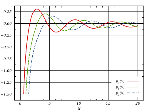
Spherical Bessel functions: $j_n\& y_n$; $h_n^{(1)}\& h_n^{(2)}$（球贝塞尔）

When solving the Helmholtz equation in spherical coordinates by separation of variables, the radial equation has the form：

$\fbox{$ x^2y''+2xy'+(x^2-n(n+1))y = 0 $}$

or, in the form of eigenvalue problem:

$y^2\dfrac{Y''}{Y} + 2y\dfrac{Y'}{Y} + y^2 = n(n+1)$

The two linearly independent solutions to this equation are called the spherical Bessel functions $j_n$ and $y_n$, and are related to the ordinary Bessel functions $J_n$ and $Y_n$ by

$j_n(x) = \sqrt{\frac{\pi}{2x}} J_{n+\frac{1}{2}}(x) \\ y_n(x) = \sqrt{\frac{\pi}{2x}} Y_{n+\frac{1}{2}}(x) = (-1)^{n+1} \sqrt{\frac{\pi}{2x}} J_{-n-\frac{1}{2}}(x)$

And we can also define the $h_n^{(1,2)}$ as the Hankel functions:

$h_n^{(1)} = j_n(x)+iy_n(x)\\ h_n^{(2)} = j_n(x)-iy_n(x)$

---

Rodrigues formuals:

$j_n(x)= (-x)^n \left(\frac{1}{x}\frac{d}{dx}\right)^n\,\frac{\sin x}{x}\\ y_n(x) = -(-x)^n \left(\frac{1}{x}\frac{d}{dx}\right)^n\,\frac{\cos x}{x}$

Notice that if we set $p$ the subscripit of the Bessel function $p = (2n+1)/2 = n+1/2$,the we get $j_n$ and $y_n$ which can be expressed in terms of $\sin x$, $\cos x$ and powers of $x$.

---

Important notes:

Spherical Bessel function can be expressed by elementary functions!!

$j_{n}(x)=\sqrt{\frac{\pi}{2 x}} J_{(2 n+1) / 2}(x)=x^{n}\left(-\frac{1}{x} \frac{d}{d x}\right)^{n}\left(\frac{\sin x}{x}\right)$

$y_{n}(x)=\sqrt{\frac{\pi}{2 x}} Y_{(2 n+1) / 2}(x)=-x^{n}\left(-\frac{1}{x} \frac{d}{d x}\right)^{n}\left(\frac{\cos x}{x}\right)$

$\begin{aligned} j_{0}(x) &=\frac{\sin x}{x} \\ j_{1}(x) &=\frac{\sin x}{x^{2}}-\frac{\cos x}{x} \end{aligned}$

---

Pictures:

Kelvin functions

Airy functions: $\mathrm{Ai}\&\mathrm{Bi}$

Airy differential equation is

$\fbox{$y'' -xy = 0$}$

In the form of eigenvalue problem:

$\dfrac{Y''}{Y}-y = 0$

---

It also satisfies the general form of the Bessel differential equation, and the solution is:

$\sqrt{x}Z_{1/3}(\frac{2}{3}ix^{3/2})$

It can be writtern in the combination of $J_{1/3}$ and $N_{1/3}$. Since the parameter contains $i$, We can use hyperbolic Bessel instead:

$\begin{aligned} \mathrm{Ai}(x) & = \dfrac{1}{\pi}\sqrt{\dfrac{x}{3}}K_{1/3}\left(\dfrac{2}{3}x^{3/2}\right)\\ \mathrm{Bi}(x)& = \sqrt{\dfrac{x}{3}}\left[I_{-1/3}\left(\dfrac{2}{3}x^{3/2}\right) + I_{1/3}\left(\dfrac{2}{3}x^{3/2}\right)\right] \end{aligned}$

---

Picture:

Comparision of differential equations for Bessel Functions

Name	Differential euation
Original Bessel	$y^2\dfrac{Y''}{Y}+ y\dfrac{Y'}{Y} + y^2 = p^2$
General Bessel	$y^2\dfrac{Y''}{Y} + y(1-2a)\dfrac{Y'}{Y} + (bcy^{c-1})^2y^2 = p^2c^2-a^2$
Hyperbolic Bessel	$y^2\dfrac{Y''}{Y}+y\dfrac{Y'}{Y}-y^2 = p^2$
Spherical Bessel	$y^2\dfrac{Y''}{Y} + 2y\dfrac{Y'}{Y} + y^2 = n(n+1)$
Kelvin	$\dfrac{Y''}{Y} +\dfrac{1}{y}\dfrac{Y'}{Y} = i$
Airy	$\dfrac{Y''}{Y}-y = 0$

Hermit function 厄米方程

Laguerre function 劳厄方程

The Equation

Lagueere polynomials are solution of the differential equation:

$\fbox{$ xy''+(1-x)y'+ny = 0 $}$

or, in the eigenvalue form:

$y\dfrac{Y''}{Y} + (1-y)\dfrac{Y'}{Y} = -n$

Laguerre polynomials

Polynomial means we can expand the solution in $a_0x^0 + a_1x^1 + a_2x^2+\cdots$. And the answer is:

$\begin{aligned} L_n(x) & = 1 - nx + \dfrac{n(n-1)}{2!}\dfrac{x^2}{2!}\dfrac{n(n-1)}{2!}\dfrac{x^2}{2!} - \dfrac{n(n-1)(n-2)}{3!}\dfrac{x^3}{3!} +\cdots+\dfrac{(-1)^nx^n}{n!}\\ & = \sum^n_{m=0}(-1)^m{\binom n m}\dfrac{x^m}{m!} \end{aligned}$

Warning: some author may omit the $1/n!$ factor.

First 3 terms of Lagueere polynomials are:

$\begin{aligned} L_0(x) & = 1\\ L_1(x) & = 1-x\\ L_3(x) & = 1-2x+x^2/2 \end{aligned}$

---

Rodrigues formula:

$L_n(x) = \dfrac{1}{n!}e^x\dfrac{d^n}{dx^n}(x^ne^{-x})$

---

Orthogonality:

$\int^\infty_0e^{-x}L_n(x)L_k(x)dx = \delta_{nk}$

Attention that the polynomials are orthogonal on $(0,\infty)$ with respect to the weight function $e^{-x}$. We can also say that $e^{x/2}L_n(x)$ are orthogonal.

---

Generating function:

$\Phi(x,h) = \dfrac{e^{-xh/(1-h)}}{1-h} = \sum^\infty_{n=0}L_n(x)h^n$

---

Recursion relations:

Associated Laguerre function 伴随劳厄方程

Differential equaion

$\fbox{$ xy''+(k+1-x)y'+ny = 0 $}$

or in the form of the eigenvalue problem:

$y\dfrac{Y''}{Y}+(k+1-y)\dfrac{Y'}{Y} = -n.$

Associated Laguerre polynomials

Actually, the associated Laguerre polynomials are the Derivatives of the Laguerre polynomials. The new polynomials are defined as:

$L_n^k(x) = (-1)^k\dfrac{d^k}{dx^k}L_{n+k}(x)$

And all of the properties of the associated Laguerre polynomial could be prooved by using the drivation of Laguerre polynomials.

Warning, again, the formulas and properties here and below will be different if some author omit $1/n!$ factor before $L_n$.

---

Rodrigues formula:

$L^k_n(x) = \dfrac{x^{-k}e^x}{n!}\dfrac{d^n}{dx^n}(x^{n+k}e^{-x})$

---

Orthogonality:

$\int^\infty_0x^ke^{-x}L_n^k(x)L_m^k(x)dx = \delta_{nm}\dfrac{(n+k)!}{n!}$

Note that now the weight function becomes to $x^ke^{-x}$.

p.s. This orthogonality is not used to normalize the function of hydrogen atom

Application in physics: Radial wave function of hydrogen atom

$-\dfrac{\hbar^2}{2m}\dfrac{1}{r}\dfrac{\partial^2}{\partial r^2}\left(rR\right) + \left[\dfrac{l(l+1)\hbar^2}{2mr^2} - \dfrac{e^2}{r}\right]R = ER$

STEP 1, subsititute $R(r)$ by:

$R(r) = \dfrac{u(r)}{r}$

Then, the differential equation becomes:

$-\dfrac{\hbar^2}{2m}\dfrac{\partial^2}{\partial r^2}u + \left[\dfrac{l(l+1)\hbar^2}{2mr^2} - \dfrac{e^2}{r}\right]u = Eu$

---

STEP 2 is to change some variables to normalize the radius and the energy. $\rho\equiv \dfrac{r}{a_0}$, where $a_0$ is the Bohr radius which is defined as:

$a_0 \equiv \dfrac{\hbar^2}{me^2}$

$\rho = \dfrac{r}{a_0}\longrightarrow -\dfrac{\hbar^2}{2m}\dfrac{\partial^2}{a_0^2\partial \rho^2}u + \left[\dfrac{l(l+1)\hbar^2}{2ma_0^2\rho^2} - \dfrac{e^2}{a_0\rho}\right]u = Eu\\ \left[-\dfrac{me^4}{2\hbar^2}\dfrac{\partial^2}{\partial \rho^2} + \dfrac{l(l+1)me^4}{2\hbar^2\rho^2} - \dfrac{me^4}{\hbar^2\rho}\right]u = Eu\\ \left[\dfrac{\partial^2}{\partial \rho^2} - \dfrac{l(l+1)}{\rho^2} + \dfrac{2}{\rho}\right]u = -\dfrac{E}{\dfrac{me^4}{2\hbar^2}}u$

And we can define the Rydberg energy:

$E_\mathrm{I} \equiv \dfrac{me^4}{2\hbar^2}$

and we have $e^2 = 2a_0E_\mathrm{i}, \dfrac{\hbar^2}{2m} = a_0^2E_\mathrm{I}$.

$\left[\dfrac{\partial^2}{\partial \rho^2} - \dfrac{l(l+1)}{\rho^2} + \dfrac{2}{\rho}\right]u = -\dfrac{E}{E_\mathrm{I}}u\\ \left[\dfrac{\partial^2}{\partial \rho^2} - \dfrac{l(l+1)}{\rho^2} + \dfrac{2}{\rho}\right]u = \lambda^2u$

Where, $\lambda$ is defined as $\lambda\equiv\sqrt{-\dfrac{E}{E_\mathrm{I}}}$. Note that $E<0$.

---

STEP 3. Not enough yet. Another substitution is needed in order to eliminate the term of $\lambda^2u$:

$u(\rho) \equiv y(\rho)e^{-\lambda\rho}$

and we get:

$\dfrac{du}{d\rho} = \dfrac{dy}{d\rho}e^{-\lambda\rho}-\lambda ye^{-\lambda\rho}\\ \dfrac{d^2u}{d\rho^2} = \dfrac{d^2y}{d\rho^2}e^{-\lambda\rho} - 2\lambda\dfrac{dy}{d\rho}e^{-\lambda\rho}+\lambda^2 ye^{-\lambda\rho}$

So the differential equation now becomes:

$\dfrac{d^2y}{d\rho^2} - 2\lambda\dfrac{dy}{d\rho} + \left[\dfrac{2}{\rho}-\dfrac{l(l+1)}{\rho^2}\right]y = 0$

---

STEP 4 is to eliminate the term of $\dfrac{l(l+1)}{\rho^2}y$. Do the substitution:

$y(\rho) = \rho^{s}q(\rho) = \rho^{l+1}q(\rho)$

and we get

$y' = (l+1)\rho^lq+\rho^{l+1}q'\\ y'' = l(l+1)\rho^{l-1}q + 2(l+1)\rho^lq'+\rho^{l+1}q''$

Actually, $s$ can also choose $s = -l$, but the solution will be diverge, so we neglect this choice.

So the differential equation becomes:

$\rho q'' + [2(l+1)-2\lambda \rho]q' + [2-2\lambda(l+1)]q = 0\\ \rho\dfrac{q''}{q} + [2(l+1)-2\lambda \rho]\dfrac{q'}{q} = -[2-2\lambda(l+1)]$

---

STEP 5: We are very close to the final answer. We just need to take care the factor $-2\lambda \rho\dfrac{q'}{q}$. We can adjust the $\rho$:

$\xi = 2\lambda\rho,\quad \rho = \dfrac{\xi}{2\lambda}$

The differential equation then becomes:

$2\lambda\xi\dfrac{d^2q}{d\xi^2} + (2\lambda)[2(l+1)-\xi]\dfrac{dq}{d\xi} = -[2-2\lambda(l+1)]\\ \xi\dfrac{d^2q}{d\xi^2} + [2(l+1)-\xi]\dfrac{dq}{d\xi} = -\dfrac{2-2\lambda(l+1)}{2\lambda}\\ \xi\dfrac{d^2q}{d\xi^2} + [(2l+1)+1-\xi]\dfrac{dq}{d\xi} = -\left[\dfrac{1}{\lambda}-(l+1)\right]$

---

Compare with the function of associated Laguerre:

$y\dfrac{Y''}{Y}+(k+1-x)\dfrac{Y'}{Y} = -n$

We set

$\begin{cases} k = 2l+1\\ n_r = \dfrac{1}{\lambda}-(l+1) \end{cases}$

Where $n_r$ is called as the “raidal quantum number”, not the principal quantum number. We can see $\lambda = \dfrac{1}{n_r+l+1}\equiv\dfrac{1}{n}$, and define $n = n_r+l+1$ which is the principal quantum number. We know that $n_r\geq 0$, so the choices examples for $n$ and $n_r$ are:

$\begin{aligned} n = 1 : & l=0, & n_r = 0 \\ n = 2 : & l=0, & n_r = 1 \\ & l=1, & n_r = 0 \\ n = 3 : & l=0, & n_r = 2 \\ & l=1, & n_r = 1 \\ & l=2, & n_r = 0 \end{aligned}$

So that:

$n_r = n-l-1$

And the solution for the $q(\xi)$ is:

$q(\xi) = L^k_{n_r}(\xi) = L^{2l+1}_{n-l-1} = q_{nl}(\xi)$

---

Finally, let’s go over the whole transmission during the derivation:

$\begin{aligned} R(r) & = \dfrac{u(r)}{r}\\ & = \dfrac{y(\rho)e^{-\lambda\rho}}{r}\\ & = \dfrac{y\left(\rho\right)e^{-\lambda r/{a_0}}}{r}\\ & = \dfrac{\rho^{l+1}q(\rho)e^{-\lambda r/{a_0}}}{r}\\ & = \dfrac{(r/a_0)^{l+1}q(\rho)e^{-\lambda r/{a_0}}}{r}\\ & = \dfrac{(r/a_0)^{l+1}q(\xi)e^{-\lambda r/{a_0}}}{r}\\ & = \dfrac{(r/a_0)^{l+1}e^{-\lambda r/{a_0}}}{r}q\left(\xi = 2\lambda\rho = \frac{2\lambda r}{a_0}\right)\\ & = \dfrac{(r/a_0)^{l+1}e^{-\lambda r/{a_0}}}{r}q\left(\frac{2\lambda r}{a_0}\right)\\ R_{nl}(r) & = \dfrac{(r/a_0)^{l+1}e^{-r/n{a_0}}}{r}q_{nl}\left(\frac{2r}{na_0}\right)\\ & = \dfrac{(r/a_0)^{l+1}e^{-r/n{a_0}}}{r}L^{2l+1}_{n-l-1}\left(\frac{2r}{na_0}\right)\\ \end{aligned}$

$\fbox{$R_{nl}(r) = \dfrac{r^l}{a_0^{l+1}}e^{-r/n{a_0}}L^{2l+1}_{n-l-1}\left(\frac{2r}{na_0}\right)$}$

Attention. the normalization of the solution is not the orthogonality above. We should use

$\int^\infty_0x^{k+1}e^{-x}[L^k_n(x)]^2dx = (2n+k+1)\dfrac{(n+k)!}{n!}$

Confluent hypergeometric function 合流超几何函数

The Kummer-Laplace Differential Equation

$\fbox{$ xy''+(c-x)y-ay = 0 $}$

or the eigenvalue problem form:

$y\dfrac{Y''}{Y} + (c-y)\dfrac{Y'}{Y} = a$

Confluent hypergeometric functions $F(a,c;x)\& G(a,c;x)$

The solution which is regular at the origin is called the confluent hypergeometric function and denoted as $F(a, c; x)$ or ${}_1F_1(a, c; x)$. Sometimes it is also called the degenerate hypergeometric function, because it can be obtained as a limiting case of a more general Gauss hypergeometric function.

Comparision of each differential special function 对比与总结

Name	differential equation
Legendre	$(1-y^2)\dfrac{Y''}{Y}-2y\dfrac{Y'}{Y} = -l(l+1)$
Associated Legendre	$(1-y^2)\dfrac{Y''}{Y}-2y\dfrac{Y'}{Y} - \dfrac{m^2}{1-y^2} = -l(l+1)$
Bessel	$y^2\dfrac{Y''}{Y}+ y\dfrac{Y'}{Y} + y^2 = p^2$
Hermite	$\dfrac{Y''}{Y} -2y\dfrac{Y'}{Y} = -2n$
Laguerre	$y\dfrac{Y''}{Y}+(1-y)\dfrac{Y'}{Y} = -n$
Associated Laguerre	$y\dfrac{Y''}{Y}+(k+1-y)\dfrac{Y'}{Y} = -n$
Confluent hypergeometric function	$y\dfrac{Y''}{Y} + (c-y)\dfrac{Y'}{Y} = a$